- Soroco Tops Everest Group’s PEAK Matrix® Assessment - Four Years in a Row
Scout
Customer Stories
Ecosystem
Work Graph
Increasing the Accuracy of Textual Data Analysis on a Corpus of 2,000,000,000 Words
Michael Lee
Response By Engineering, SRE, and Customer Success
- 4 December 2021
- 14 minute read
Introduction
Natural language processing (NLP) is one of the most active subfields of machine learning today. Text classification, topic modeling, and sentiment analysis have become vital techniques in a myriad of real-world technological applications, such as search engine optimization and content recommendation. E-mails, social media posts, news articles, and other documents are constantly mined for insights on human opinions and behaviors by scientists, large and small companies, and even state actors.
At Soroco, natural language processing and machine learning-based classification of text are foundational to many of our products. In some instances, we may ingest between 200,000,000 and 2,000,000,000 words over the course of model training and analysis for a single team of workers using our Scout product. In this blog post, we will address some tips and tricks which we have found to significantly increase the accuracy of our models, including appropriate processing of text for the purpose of leveraging standard techniques from machine learning. Many advanced methods for performing text classification require careful modifications so as to respect the structure of multi-field textual data for optimal performance.
To illustrate the benefits of these techniques, this two-part series of blog articles will demonstrate the following ideas:
- We will show how to represent text in a high-dimensional vector space with applications to a toy regression problem.
- We will detail how to perform multi-field textual data analysis using more sophisticated neural network technologies.
Challenges of Text Analysis
Text analysis is complicated by the variety of nuance inherent in each application: real-world problems in NLP require analyzing complicated bodies of text, such as ones which are split into multiple fields or contain many words of natural language.
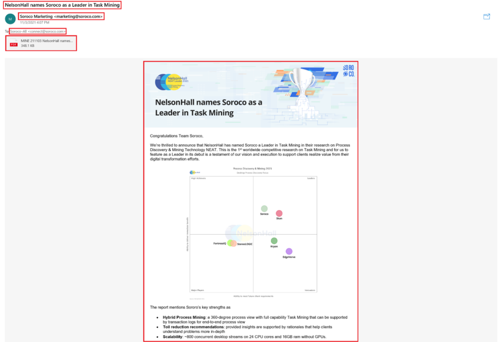
Text fields in an email may include the subject, the sender and recipient, the email body, and the contents of any possible attachments.
To illustrate the challenges and important aspects of modern text classification, we have included a sample e-mail where Soroco’s marketing team announced NelsonHall naming Soroco as a leader in Task Mining.
This e-mail, like any other, has multiple text fields. Based on the text of the e-mail body, its subject line, and the identities of its senders and recipients, we may wish to perform some kind of classification task. For example, we may want to classify the e-mail as a “Positive Announcement,” or detect that it’s related to marketing.
However, how do we properly set up a model to classify this email correctly and efficiently? Here are some potential challenges we might run into as we train a model to identify “Positive Announcement” emails:
- We might be tempted to take the entire text and collapse it into a single block of text for the classifier. However, that would cause all fields to be weighted with equal importance, which is not the case. For example, for this task in particular, the presence of positive words such as “Congratulations” in the email’s subject might be more pertinent than the content of the email body.
- What if all e-mails passed to the classifier in training always had the opening “Congratulations to the Soroco Team”, but a future email began as “Kudos to the Soroco Team”? The input to the model during training and classification (e.g., how words are vectorized) can have a significant impact on the accuracy of the classification.
- Once we’ve vectorized the text fields appropriately, there are many different classifier types we might use to solve the classification problem. However, not all of them will necessarily perform well with our chosen vectorization method. Some classifiers may work better with fasttext or word2vec embeddings (which tend to produce dense, high-dimensional output), whereas others might work with tf–idf mappings (which are sparse but can be of much higher dimension depending on your corpus). Some experimentation may be required to find the model architecture that performs best for our input.
In Part 1 of this blog article, we are going to first address the importance of the vectorization of words and show how this vectorization has implications on the model’s accuracy and performance. In the second article, we will show further illustrate the importance of training on multiple fields and the impact to the model.
Building a Model with Word Embeddings
The approaches we cover here are going to rely on the concept of a latent embedding of textual data into a vector space, such as through word embeddings. Although there are simpler statistical methods for doing basic NLP, such as tf–idf, for our purposes we prefer a method where we assign some notion of semantic significance to our data. This semantic significance is the key to making the model resilient to the many ways in which the same contextual meaning can be written (i.e., like “congratulations” and “kudos” in our example above).
Word embeddings provide a vector space representation of each word in a vocabulary such that words which appear in similar contexts (such as synonyms) have representations which are close together in space. This helps us to be robust against the variation in word choice we might see in real-world applications, where we are trying to analyze textual data produced by people.
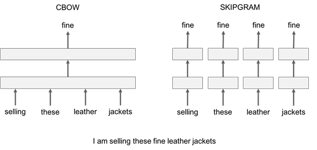
From fasttext.cc
The above diagram from Facebook Research shows the difference between two strategies for optimizing word embeddings. In the CBOW (“continuous bag of words”) approach, we train a network to predict the embedding of a word from the sum of embeddings of all words within a fixed-size window around that word. In the sample sentence, “I am selling these fine leather jackets,” the embedding of the word “fine” is predicted from the sum of the embeddings of the words “selling,” “these,” “leather,” and “jackets.” In contrast, in the skipgram approach, we train the network to predict the embedding of a word from a random word selected from that fixed-size window, so the embedding of the word “fine” is predicted from the embedding of one of the words “selling,” “these,” “leather,” or “jackets” on subsequent training epochs.
The first decision to make is what kind of word embeddings we want to use for encoding our text data. There are several existing implementations of word embeddings for us to choose from, but the two styles we will consider are word2vec and fasttext. The main difference between these is how a morpheme is defined in each. The simpler method is word2vec: every word gets its own word vector. With fasttext, we take the more granular approach of considering subword-level information by assigning additional semantic significance to “character n-grams,” or groupings of a fixed number of consecutive characters within a word. By considering these character n-grams, we can generate a fasttext word vector for a word which does not appear in the training corpus. This allows us to better compensate for things like slight misspellings, as well as conjugation and declension (particularly in languages with many verb tenses or noun cases, where we might want inflections of the same word class to be grouped closely by our embedding).
Facebook makes pretrained fasttext models available for 157 languages, trained using corpuses dumped from Common Crawl and Wikipedia. These are useful in cases where we may not have access to enough textual data to train our own word embeddings. In the following demonstration, we will train a fasttext model (Facebook Research provides a tutorial with more information on how to do this) and use it to try to solve a nontrivial textual analysis problem.
Demonstration
Let’s define a toy regression problem with some textual inputs: Choose some type of product (let’s say books, for the purpose of our demonstration). Using all the reviews and ratings assigned by one book reviewer to a selection of books, can we predict what rating a previously unseen book might receive from the reviewer given only its description?
Our toy dataset will consist of all the reviews published on Goodreads by one of the site’s most prolific reviewers. For the purpose of this demonstration, we will take the following naïve approach. First, we define a book pair, where we have access to the book description, review text, average rating, and personal rating for one book (the “reviewed book”) and only the book description and average rating for the other book (the “unreviewed book”). Our model input will therefore consist of some vector representation of the descriptions of both books, as well as the review text for the reviewed book. In order to pass all this information to the model, we separately vectorize each text field, then concatenate the resulting vectors (we get much worse results by attempting to concatenate the text fields for the reviewed book before vectorizing; this points to some additional value for the model in being able to distinguish between the book’s objective description and the reviewer’s take on the book). The desired model output will be number capturing the reviewer’s bias in rating the unreviewed book, relative to their bias in rating the reviewed book. We calculate this as the signed difference between the personal and average ratings for the reviewed book, minus the signed difference between the personal and average ratings for the unreviewed book. Although a reviewer’s take on an individual book might not be predictive of their feelings about another arbitrary book in the general case, we can get a better picture of the reviewer’s biases by averaging our model output over all the reviewed books in the training dataset in predicting their rating of each book in the test dataset. A more sophisticated approach to this might be to take a weighted average, where the weights correspond to some measure of similarity between the book descriptions (or subject classifications, if we additionally have access to this data).
First, we aggressively preprocess our text so that everything is lower-cased and punctuation, extra whitespace, and purely numeric tokens are stripped out:
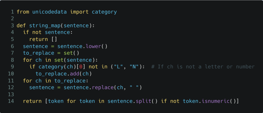
We split our data into a training set and a validation set:
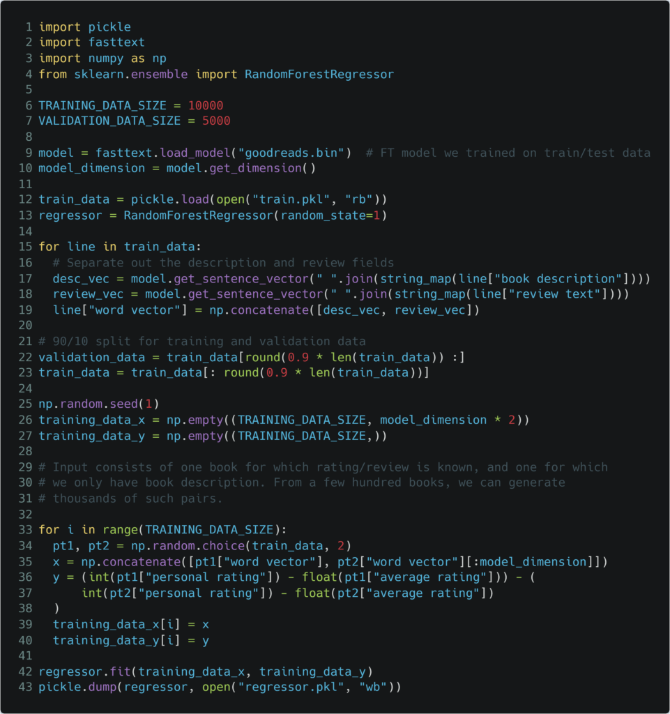
We will measure the quality of our regressor as the R2 score (or coefficient of determination) of the regressor’s predictions on the validation set with respect to the ground truth:
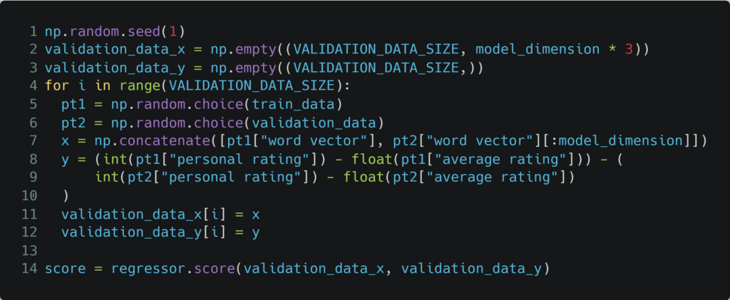
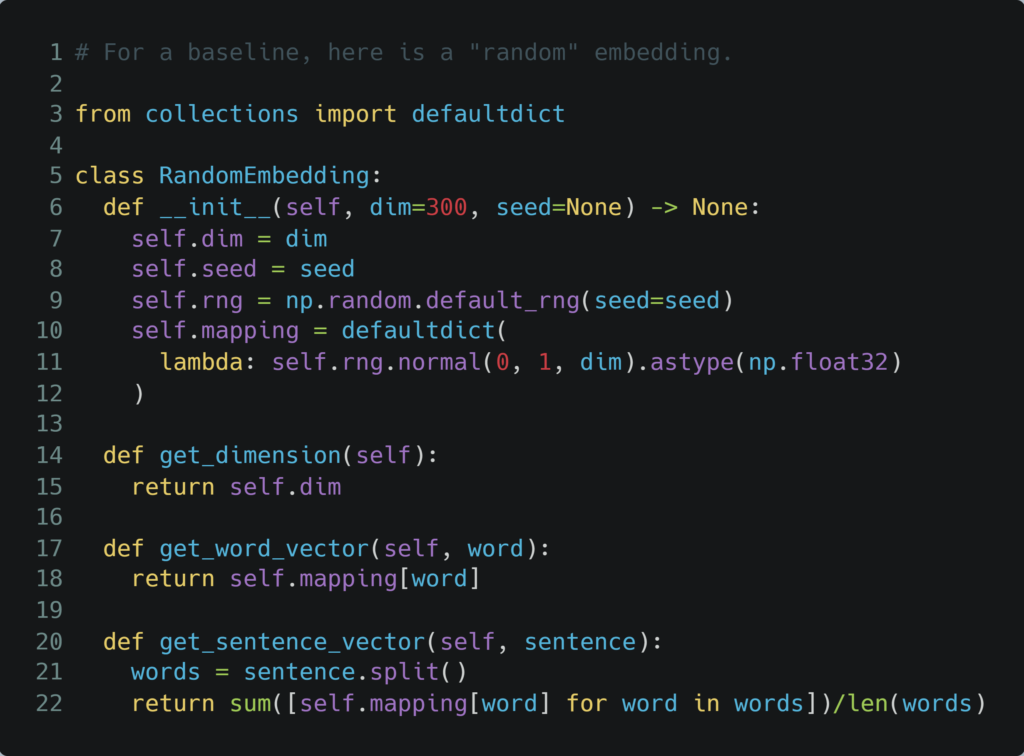
You can see the results of our demonstration in this Google Colab notebook. The most common approach to calculating the vector representation of a sentence using word embeddings is to remove stopwords (such as articles, conjunctions, and prepositions) and then to take the mean of the remaining word vectors. We find that we can increase the R2 score of our model by instead providing as input the “bounding box” of the word vectors, which consists of the minimum and maximum value over all words in a sentence along each axis in the space of embeddings. Even though we are effectively doubling the number of input features we are providing to our model (possibly inviting overfitting), we do end up improving the fit of our model on our validation data.
To show the advantages of word embeddings with semantic content on difficult NLP problems like our toy problem, we can attempt to solve the same problem with tf–idf vectorizations of the same textual data fields. With LASSO regression, we can mitigate some issues created by the number and sparsity of features resulting from our tf–idf mapping (notably, the random forest models we have been using up to this point perform inefficiently with sparse features due to the fact that each estimator in the forest only “sees” a small fraction of the available features by default; furthermore, the input matrix must be un-sparsified in order to be used with the sklearn random forest implementation, which can lead to memory issues if we have a large number of distinct tokens represented by our tf–idf mapping). However, we find that our fit is still much lower quality than those generated using our word embedding strategy:
| Method | R² Score, Test Set |
|---|---|
| Fasttext embeddings (one field), RF regression | 0.322 |
| Random embeddings (separate fields) | 0.320 |
| Fasttext embeddings (separate fields, sentence average) | 0.392 |
| Fasttext embeddings (separate fields, sentence bounding box) | 0.418 |
| tf–idf, LASSO regression | -0.020 |